Structured prediction

baseNP: doesn’t contain any recursive parts.

chunking: build the tree for the sentence

Level of representation:

* Brown Corpus (level1: pos)

* Penn Trecbank (level2: sys)

* PropBank (level3: sen)

* Framenet (level4: )

All of these need lots of human labor.


h(x) = argmin(y in Y) E_(y~p(Y|X))[l(y,x,Y)]

l (y*,x,y) = 1 – delta(y,y*)

H(x) = argmax_(y in Y) Pr(y|x)

min_(h in H) E_{p}[loss(X;Y;h)] + model complexity(h)

Empirical risk = 1/N SUM_{I = 1}^{N}loss(x,y*,h)


generalized viterbi

recognize speech

wreak a nice beach

an ice beach


conditional random fields

Lecture 10: Neural Network

  1. Deep learning
  2. Representation learning
  3. Rule-based
    1. high explainability
  4. Linguistic supervision
  5. Semi-supervision
    1. have small set of data with label
    2. has large set of data without label
  6. Recurrent-level supervision
  7. Language structure

description lengths DL= size(lexicon) + size( encoding)

  1. lex1
    1. do
    2. the kitty
    3. you
    4. like
    5. see
  2. Lex2
    1. do
    2. you
    3. like
    4. see
    5. the
    6. kitty
  3. How to evaluate the two lexicons?
    1. lex 1 have 5 words, lex 2 has 6 words
    2. Potential sequence
      1. lex1: 1 3 5 2, 5 2, 1 3 4 2
      2. lex2: 1 3 5 2 6, 5 2 6, 1 3 4 2 6
  1. MDL: minimum description lengths
    1. unsupervised
    2. prosodic bootstrapping

Boltzmenn machine

Lexical space

relatedness vs. similarity

  • use near neighbors: similarity
  • use far neighbors: relatedness

ws-353 has similarity & relatedness

loss function:


project:

Part1: potential methods

  • LDA
  • readability
  • syntactic analysis


Word2Vec Models

Collection of all pre-trained Word2Vec Models:

http://ahogrammer.com/2017/01/20/the-list-of-pretrained-word-embeddings/

Google’s model seems not reliable…

Here are some similarity tests of Google’s model:

The similarity between good and great is: 0.7291509541564205
The similarity between good and awesome is: 0.5240075080190216
The similarity between good and best is: 0.5467195232933185
The similarity between good and better is: 0.6120728804252082
The similarity between great and awesome is: 0.6510506701964475
The similarity between great and best is: 0.5216033921316416
The similarity between great and better is: 0.43074460922502006
The similarity between awesome and best is: 0.3584938663818339
The similarity between awesome and better is: 0.27186951236001483
The similarity between best and better is: 0.5226434484898708
The similarity between food and foodie is: 0.3837408842876883
The similarity between food and eat is: 0.5037572298482941
The similarity between foodie and eat is: 0.3050075692941569
The similarity between park and view is: 0.1288395798972001
The similarity between design and art is: 0.3347430713890944

Lecture 8: Evaluation

  • Information about midterm
  • PCFG
    • Start with S
    • ∑Pr(A -> gamma | A) = 1
      • (conditional) probability of each item has to sum to one
    • Pr(O = o1,o2,…,on|µ)
      • HMM: Forward
      • PCFG: Inside-Outside
    • Guess Pr: argmax_(Z)[ Pr(Z|O, µ) ]
      • HMM:Use Viterbi to get
      • PCFG: Use Viterbi CKY to get
      • *Z is the best sequence of states
    • Guess µ: argmax_(µ)[Pr(O|µ)]
      • HMM:Use forward-backward to get
      • PCFG: Use Inside-outside to get
    • Example:
      • Sentence:
        • ——————-S
        • ——–NP—————-VP
        • ——–NP———-V————-NP
        • ——people——eats —–adj——–N
        • —————————roasted—-peanuts
      • Problem:
        • Pr_µ(peanuts eat roasted people) = Pr_µ(people eat roasted peanut)
      • We can try to generate head of each phrase:
        • ————————————S (Head: eat)
        • ——–NP(Head: people)—————————–VP(Head: eat)
        • ——–NP(Head: people)———-V(Head: eat)——————————–NP(Head: peanut)
        • ——people(Head: people)——eats(Head: eat)————-adj(Head: N/A)—————–N(Head: peanut)
        • —————————————————————–roasted(Head: N/A)————-peanuts(Head: peanut)
      • Should have: Pr[S (Head: eat) -> NP(Head: people) VP(Head: eat)] > Pr[ S (Head: eat) -> NP(Head: peanut) VP(Head: eat) ]
    • Dependency representation:
      • Sentence:
        • —————————eat
        • —————people—————peanuts
        • —————–the—————–roasted
      • Lexical (bottom up)
      • NP ->det N
  • Evaluation
    • Reference Reading:How Evaluation Guides AI Research
      • Intrinsic evaluation
      • Extrinsic evaluation
    • Kappa’s evaluation
    • Metric: precision recall
    • How to evaluate two structures which could generate the same sentence?
      • Answer: Generate more than one output for each input, convert the output into set of output, and use precision and recall to measure.
    • Reader evaluation:
      • If the reader’s score agree with the machine, stop
      • else: let another reader read the essay

Lecture 6: Context-free parsing

Questions:

  1. Generative Model P(X,Y)
  2. Discriminative model P(Y|X)

MainPoints

  1. Block sampler: Instead of sample one element at a time, we can sample a batch of samples in Gibbs Sampling.
  2. Lag and Burn-in: can be viewed as parameters (we can control the number of iterations)
    1. lag: mark some iterations in the loop as lag, then throw away the lag iterations, then the other samples become independent.
      1. Example: run 1000 iters -> run 100 lags -> run 1000 iters -> 100 lags …
    2. burn in: throw away the initial 10 or 20 iterations (burn-in iterations), where the model has not converged.
      1. The right way is to test whether the model has converged.
  3. Topic model:
  4. The sum of the parameter of each word in a topic doesn’t need to be one
  5. The derivative (branches) of LDA (Non-parametric model):
    1. Supervised LDA
    2. Chinese restaurant process (CRP)
    3. Hierarchy models
      1. example: SHLDA
      2. gun-safety (Clinton) &  gun-control (Trump)

Parsing:

Any context which can be processed with FSA can be processed with CFGs. But not vice versa.

? turning machine
 (Don’t cover in this lecture)
CSL Tree adjusting Grammar PTAGs
 (Don’t cover in this lecture)
CF PDA/CFGs PCFGs
PDA/CFGs Allow some negative examples. And can handle some cases that cannot be processed by FSA.

For example: S -> aSb {a^nb^n} cannot be processed by FSA because we need to know the variable n. But FSM only remember the states, it cannot count.

Regular FSA/regular expressions HMM

Example1:

The rat that the cat that the dog bit chased died.

Example2:

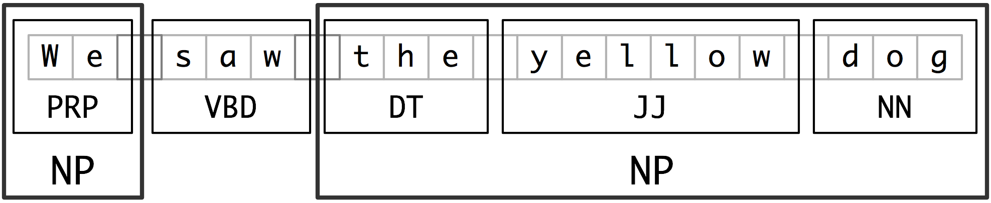
Sentence: The tall man loves Mary.

————-loves

—–man————Mary

-The——tall

Structure:

——————-S

——–NP——————VP

—DT-Adj—N             V——–NP

—the-tall–man       loves—–Mary

Example3: CKY Algorithm

0 The 1 tall 2 man 3 loves 4 Mary 5

[w, i, j] A->w \in G

[A, i, j]

Chart (bottom up parsing algorithm):

0 The 1 tall 2 man 3 loves 4 Mary 5

–Det —— N ———V ——NP—-

———–NP ———–VP ———

—————- S ———————

Then I have:

[B, i, j]

[C, j, k]

So I can have:

A->BC : [A, i, k] # BC are non-determinal phrases

NP ->Det N

VP -> V NP

S -> NP VP

Example4:

I      saw         the        man       in        the       park        with      a       telescope.

——————– NP—————– PP ———–

–                         —————NP———————

————————NP—————————–


A->B . CD

B: already

CD: predicted

[A -> a*ß, j]

[0, S’-> *S, 0]

scan: make progress through rules.

[i, A -> a* (w_j+1) ß, j]

A [the tall] B*C

i, [the tall], j

Prediction: top-down prediction B-> γ

[i, A-> a * Bß, j]

[j, B->*γ, j]


Combine

Complete (move the dot):

[i, A->a*ß, k] [k, B->γ, j]


I                          k                       j

–[A->a*Bß]———[B->γ*]—–


Then I have:

[I, A->aB*ß, k]

Lecture 5: Reduced-dimensionality representations for documents: Gibbs sampling and topic models

    • watch the new talk and write summary
    • Noah Smith: squash network
    • Main points:
      • difference between LSA & SVD
      • Bayesian graphical models
        • informative priors are useful in the model
      • Bayesian network
        • DAG
        • X1X2…Xn
        • Po(X1, X2, …, Xn)
        • Generative story: HMM (dependencies)
        • A and B are conditionally independent given C iff P(A,B|C) = P(A|C) * P(B|C)
          •       C (to A, to B)
          •   A                             B
        • Example:
          •               Cloudy (to Sprinter and rain)
          • Sprintder(to wet grass)                   Rain (to wet grass)
          •                       Wet grass(final state)
          • w’s are observable
          • State change graph:  π -> S1 -> S2 -> S3 -> … -> St
          • w’s are observable
            • μ~(A,B,π)
            • Have a initial π for C, π~Beta(Gamma(π1), Gamma(π2))
            • C is Bernoulli (π)
            • S~ Bernoulli(π(S | C))
            • R~Bernoulli(π(S | C))
            • W ~ Bernoulli(\tao (ω | S,R))
            • π~Dirichlet(1)
            • S1~Cat(π)S2~Cat(a_s1,1  ,  a_s1,2  ,   ….  ,   a_(s1,n))* Cat is chosen from the transition matrix
            • ω1~Cat(b_s1,1  ,  b_s1,2  ,   ….  ,   b_(s1,n))ω2~Cat(b_s1,1  ,  b_s1,2  ,   ….  ,   b_(s1,n))* Cat is chosen from the transition matrix
        • What just been introduced is the unigram model, here is the bigram model
        • P(s1, s2, …. , sn) = P(s1) P(s2|s1) P(s3|s1,s2) P(s4|s2,s3)..
        • For EM, we need to recalculate everything, conditional distribution are different
      • Some distributions:
        • Binomial vs. Bernoulli
        • Multinomial vs. discrete / categorical
    • Document squashing

    Continue reading Lecture 5: Reduced-dimensionality representations for documents: Gibbs sampling and topic models

Lecture3: Information Theory

  • Today’s class is about:
    • Hypothesis testing
    • collocations
    • Info theory
  • Hypothesis Testing
    • Last lecture covered the methodology.
  • Collocation
    • “religion war”
    • PMI, PPMI
      • PMI = pointwise mutual information
        • PMI = log2(P(x,y)/(P(x)P(y))) = I(x,y)
      • PPMI = positive PMI = max(0, PMI)
        • Example: Hong Kong, the frequency of “Hong” and “Kong” are low, but the frequency for “Hong Kong” is high.
      • Non-statistical measure but very useful: Not a classic hypothesis testing.
      • Note: If the frequency of the word is less than 5, then even if the PMI is high, the bigram is meaningless.
    • RFR
      • rfr(w) = (freq(w in DP)/(#DP))/(freq (w in background corpus)/(#background corpus))
      • DP is an child class in background corpus.
    • Chi-square test
      • Draw the table is important.
    • T-test
      • Non-statistical measure but very useful.
        • Not a classic hypothesis testing.
      • sliding window scan the sentence to find the bigram.
        • found ->1
        • not found ->0
      • A fox saw a new company’s emerge…..
        • A fox ->0
        • fox saw -> 0
        • saw a ->0
        • a new -> 0
        • new company -> 1
        • company emerge -> 0
  • Info theory
    • Entropy: degree of certainty of X; information content of X; pointwise information of X; (ling) surprisal, perplexity
      • X~P, H(X) = E[-log2(p(x))] = -sum(p(x)log2(p(x)))
      • H(X,Y) = H(X) + H(Y) – I(X, Y)
        • H(X, Y) is the cost of communicating between X and Y;
        • H(X) is the cost of communicating X;
        • H(Y) is the cost of communicating Y;
        • I(X, Y) is the saving because X and Y can communicate with each other.
    • Example: 8 horses run, the probability of winning is:
      • horse:    1  .     2   .   3   .    4   .    5   .   6   .     7   .       8
      • Prob:    1/2, 1/4   , 1/8,  1/16, 1/32, 1/64, 1/128, 1/256
      • Code1:   000, 001, 010,  011,   100,  101,     110,      111
        • H(X) = 3;
      • Code2:0, 10, 110,  1110,  111100, 1111101, 111110, 111111
        • Huffman code.
        • H(X) = 2;
    • Structure
      • [W -> encoder] -> X-> [                    ]->    Y  -> [decoder  -> W^]
      •        Source                    channel (P(y|x))
      • Anything before Y is the noisy channel model.
      • P(X,Y) is the joint model, P(X|Y) discriminative model.
      • T^ (estimated T)
        • =argmax_T (P(T|W))
        • = argmax_T(P(W|T)P(T)/P(W))
        • = argmax_T(P(W|T)P(T)) (W can be omitted because its’s just a scaler)
        • = argmax_T(P(w1|t1)P(w2|t2)…p(w.n|t.n) P(t1)P(t2|t1)P(t3|t2,t1)…P(tn|t1,t2, …, t.n-1))
        • = argmax_T(P(w1|t1)P(w2|t2)…p(w.n|t.n) P(t1)P(t2|t1)P(t3|t2)…P(t.n))
      • E^ = argmax P(F|E)P(E)
        • F = French, E = English, translation from English to French.
    • Relative entropy: KL divergence
      • We have an estimated model q and a true distribution p
      • D(p||q) = sum_x(p(x).log(p(x))/ log(q(x)))
      • Properties:
        • D(p||q) >= 0, equal is true when p == q
        • D(p||q) != D(q||p)
        • D(p||q) = E_p[p(x)] – E_p[q(x)]   E_p(q(x)) is the cross entropy
      • Example:
        • Model q: P(X)P(Y) independent
        • truth   p: Q(X, Y) joint
        • D(p||q)
          • = sum_x,y [p(x,y) log2(p(x,y)/p(x)p(y))]
          • = E_x,y [log2(p(x,y)/p(x)p(y))] average mutual info is the expectation of pointwise mutual info
    • Cross entropy: (perplexity)
      • Question: how good is my language model? How do I measure?
      • p(w1, w2, w3, w4) = p(w1) p(w2|w1) … p(w4|w1 w2 w3)
        • p(w4|w1 w2 w3) = p(w4|w*, w2 w3)
        • make it Markov, and combine everything beside the prev and the prev-prev.
      • D(p||m) = sum[p(x.1 … x.n)log(p(x.1 … x.n)/m(x.1 … x.n))]
        • but how do you know the truth?
        • what if n is very large?
      • H(p,m)=H(p) + D(p||m)  = -sum[p(x)log(m(x))]
        • H(p,m) can be an approximation of D(p||m), then:
        • We can sample from p and check H(p,m) by the samples, then:
        • H(L,m) = lim_(n->infinity) [- 1/n sum(p(x.1 … x.n)log(m(x.1 … x.n)))], then:
        • we need p(x.1 … x.n) be a good sample of L.
        • H(L,m) = lim_(n->infinity) [1/n log m(x.1 … x.n)]
        • m(x.1 … x.n) = product(m(x.i| x.i-1))
        • If m(*) = 0 -> H(p,m) = infinity
        • Should associate the cost with something…
          • smoothing (lots of ways for smoothing)
    • Perplexity:
      • 2^(H(x.1 … x.n, m)) i.e. 2^ (cross entropy)
      • effective vocabulary size
      • recover the unit from “bits” to the original one.

After class (M& S book)

  • 6.2.1 MLE: gives the highest probability to the training corpus.
    • C(w1, … ,wn) is the frequency of n-gram w1…wn in the training set.
    • N is the number of training instances.
    • P_MLE(w1, …, wn) = C(w1, … , wn) / N
    • P_MLE(wn | w.1, …, w.n-1) = C(w1, … , wn)/C(w1, … , w.n-1)
  • 6.2.2 Laplace’s law, Lidstone’s law and the Jeffreys-Perks law
    • Laplace’s law
      • original smoothing
      • Lidstone’s law
      • Jeffreys-Perks law
        • Expected likelihood estimation (ELE)
  • 6.2.3 Held Out Estimation
    • Take further test and see how often bigrams that appeared r times in the training text tend to turn up in the future text.
  • 6.2.4 Cross Validation
    • Cross validation:
      • Rather than using some of the training data only for frequency counts and some only for smoothing probability estimates, more efficient schemes are possible where each part of the training data is used both as initial traiining data and as held out data.
      • Deleted Estimation: two-way cross validation:

Lecture 2: Lexical association measures and hypothesis testing

Pre-lecture Readings.

  • Lexical association
    • Named entities: http://www.nltk.org/book/ch07.html
      • Information extraction architecture
        • raw text->sentence segmentation->takenization0<part of speech tagging->entity detection->relation detection
        • chunking: segments and labels multi-token sequences as illustrated in 2.1.../images/chunk-segmentation.png
          • Noun-phrase (NP) chunking
          • tag patterns: describe sequences of tagged words
          • Chunking with Regular Expressions
          • Exploring Text Corpora
        • Chinking: define a chink to be a sequence of tokens that is not included in a chunk
        • Representing chunks: tags & trees
        • Training Classifier-Based Chunkers
    • Accurate methods for the statistics of surprise and coincidence
  • An introduction to lexical association measures:
    • We use the term lexical association to refer to the association between words.
    • 3 types of association:
      • collocational association: restricting combination of words into phrases
      • semantic association: reflecting the semantic relationship between words
      • d cross-language association: corresponding to potential translations of words between different languages
  • Topics:
    • Knowledge/ data->zipf
    • Hypothesis testing
    • Collations
    • NER
  • Knowledge/ data
    • Rationalist:
    • Empiricist: driven by observation
    • Zipf’s law: the frequency of any word is inversely proportional to its rank in the frequency table.
      •                                      Empiricist                          Rationalist
      • core                              frequent
      • periphery                     infrequent                     exception relation
    • Example 1
      • Alice like it. a book.
      • Question: what does Alice like?
      • Instead of using a string of word, use a tree structure to represent a sentence.
      •              CP
      •    spec           IP
      • what         Alice like
    • Example 2 (Rationalist)
      • Which book did mary say that Bill thinks Alice like?
      • He dropped a book about info theory.
      • What did he drop a book about? (questionable) What did he write a book about? (Good)
      • He dropped [a book about info theory].
      • S                                   NP
    • Example 3
      • What does Mary read?
      •        SBarQ
      • WhNP                             SQ
      • WP           VR           NP             VBR                   NP
      •  what         odes     mary              read                  T*-1
    • Balance between rationalist and empiricist
    • Accuracy vs. coverage
    • Data-driven algorithms less concerned with over generation
    • Semi-supervised learning
    • How to relate the algorithm to the wat we learned.
    • 80-20 rule
    • Remove the low-frequency word and focus on the frequent words for the structure.
  • Hypothesis testing (Chi^2 test)
    • P(H|E) H: hypothesis, E: evidence
    • P(q = 0.7 | 76 success, 24 failures)
    • pmf:
    • R = P(H1|E) / P(H2|E)
    • Recipe for statistical hypothesis
      • Step 1: H0: null hypothesis (what we think is not true)
        • Example: coin flip: coin has only one side.
      • Step 2: Test statistic: number we compute based on evidence collection
      • Step 3: Identify test statistics distribution: if H0 were true.
      • Step 4: Pick a threshold to convince that the H0 is not true.
      • Step 5: Do an experiment and calculate the test statistic.
      • Step 6: If it sufficiently improbable assuming H0 is true, should reject H0.
        • H0: q = 0.05, H1: q != 0.05
    • Example:
      • H0: P(H) = 0.05
      • R~Binomial(n, p)
      • Likelihood func: b(r,n,p) = C(n r) p^r (1-p)^(n-r)
      • Test statistics: # heads
      • Threshold:
        • alpha = 10e-10 Type II: “miss”, “false negative”
        • alpha = 0.2 Type I: “false positive”
        • Typically, people choose alpha = 0.05
      • The value on the edge (alpha = 2.5%) is critical value.
      • Tips:
        • alpha is selected in advance. (p-hacking)
        • Cannot be used to prove something is true, only can show that something is not true.
        • Chi^2? X^2
    • Difference between Chi^2 test and T-test
    • How do I know how many times of experiment is convincing?
    • Collocation:  collocation is a sequence of words or terms that co-occur more often than would be expected by chance.
      • Kict the bucket = to die