Author: xiaoxumeng

• Today’s class is about:
  • Hypothesis testing
  • collocations
  • Info theory
• Hypothesis Testing
  • Last lecture covered the methodology.
• Collocation
  • “religion war”
  • PMI, PPMI
    • PMI = pointwise mutual information
      • PMI = log2(P(x,y)/(P(x)P(y))) = I(x,y)
    • PPMI = positive PMI = max(0, PMI)
      • Example: Hong Kong, the frequency of “Hong” and “Kong” are low, but the frequency for “Hong Kong” is high.
    • Non-statistical measure but very useful: Not a classic hypothesis testing.
    • Note: If the frequency of the word is less than 5, then even if the PMI is high, the bigram is meaningless.
  • RFR
    • rfr(w) = (freq(w in DP)/(#DP))/(freq (w in background corpus)/(#background corpus))
    • DP is an child class in background corpus.
  • Chi-square test
    • Draw the table is important.
  • T-test
    • Non-statistical measure but very useful.
      • Not a classic hypothesis testing.
    • sliding window scan the sentence to find the bigram.
      • found ->1
      • not found ->0
    • A fox saw a new company’s emerge…..
      • A fox ->0
      • fox saw -> 0
      • saw a ->0
      • a new -> 0
      • new company -> 1
      • company emerge -> 0
• Info theory
  • Entropy: degree of certainty of X; information content of X; pointwise information of X; (ling) surprisal, perplexity
    • X~P, H(X) = E[-log2(p(x))] = -sum(p(x)log2(p(x)))
    • H(X,Y) = H(X) + H(Y) – I(X, Y)
      • H(X, Y) is the cost of communicating between X and Y;
      • H(X) is the cost of communicating X;
      • H(Y) is the cost of communicating Y;
      • I(X, Y) is the saving because X and Y can communicate with each other.
  • Example: 8 horses run, the probability of winning is:
    • horse:    1  .     2   .   3   .    4   .    5   .   6   .     7   .       8
    • Prob:    1/2, 1/4   , 1/8,  1/16, 1/32, 1/64, 1/128, 1/256
    • Code1:   000, 001, 010,  011,   100,  101,     110,      111
      • H(X) = 3;
    • Code2:0, 10, 110,  1110,  111100, 1111101, 111110, 111111
      • Huffman code.
      • H(X) = 2;
  • Structure
    • [W -> encoder] -> X-> [                    ]->    Y  -> [decoder  -> W^]
    •        Source                    channel (P(y|x))
    • Anything before Y is the noisy channel model.
    • P(X,Y) is the joint model, P(X|Y) discriminative model.
    • T^ (estimated T)
      • =argmax_T (P(T|W))
      • = argmax_T(P(W|T)P(T)/P(W))
      • = argmax_T(P(W|T)P(T)) (W can be omitted because its’s just a scaler)
      • = argmax_T(P(w1|t1)P(w2|t2)…p(w.n|t.n) P(t1)P(t2|t1)P(t3|t2,t1)…P(tn|t1,t2, …, t.n-1))
      • = argmax_T(P(w1|t1)P(w2|t2)…p(w.n|t.n) P(t1)P(t2|t1)P(t3|t2)…P(t.n))
    • E^ = argmax P(F|E)P(E)
      • F = French, E = English, translation from English to French.
  • Relative entropy: KL divergence
    • We have an estimated model q and a true distribution p
    • D(p||q) = sum_x(p(x).log(p(x))/ log(q(x)))
    • Properties:
      • D(p||q) >= 0, equal is true when p == q
      • D(p||q) != D(q||p)
      • D(p||q) = E_p[p(x)] – E_p[q(x)]   E_p(q(x)) is the cross entropy
    • Example:
      • Model q: P(X)P(Y) independent
      • truth   p: Q(X, Y) joint
      • D(p||q)
        • = sum_x,y [p(x,y) log2(p(x,y)/p(x)p(y))]
        • = E_x,y [log2(p(x,y)/p(x)p(y))] average mutual info is the expectation of pointwise mutual info
  • Cross entropy: (perplexity)
    • Question: how good is my language model? How do I measure?
    • p(w1, w2, w3, w4) = p(w1) p(w2|w1) … p(w4|w1 w2 w3)
      • p(w4|w1 w2 w3) = p(w4|w*, w2 w3)
      • make it Markov, and combine everything beside the prev and the prev-prev.
    • D(p||m) = sum[p(x.1 … x.n)log(p(x.1 … x.n)/m(x.1 … x.n))]
      • but how do you know the truth?
      • what if n is very large?
    • H(p,m)=H(p) + D(p||m)  = -sum[p(x)log(m(x))]
      • H(p,m) can be an approximation of D(p||m), then:
      • We can sample from p and check H(p,m) by the samples, then:
      • H(L,m) = lim_(n->infinity) [- 1/n sum(p(x.1 … x.n)log(m(x.1 … x.n)))], then:
      • we need p(x.1 … x.n) be a good sample of L.
      • H(L,m) = lim_(n->infinity) [1/n log m(x.1 … x.n)]
      • m(x.1 … x.n) = product(m(x.i| x.i-1))
      • If m(*) = 0 -> H(p,m) = infinity
      • Should associate the cost with something…
        • smoothing (lots of ways for smoothing)
  • Perplexity:
    • 2^(H(x.1 … x.n, m)) i.e. 2^ (cross entropy)
    • effective vocabulary size
    • recover the unit from “bits” to the original one.

After class (M& S book)

• 6.2.1 MLE: gives the highest probability to the training corpus.
  • C(w1, … ,wn) is the frequency of n-gram w1…wn in the training set.
  • N is the number of training instances.
  • P_MLE(w1, …, wn) = C(w1, … , wn) / N
  • P_MLE(wn | w.1, …, w.n-1) = C(w1, … , wn)/C(w1, … , w.n-1)
• 6.2.2 Laplace’s law, Lidstone’s law and the Jeffreys-Perks law
  • Laplace’s law
    • original smoothing
    • Lidstone’s law
    • Jeffreys-Perks law
      • Expected likelihood estimation (ELE)
• 6.2.3 Held Out Estimation
  • Take further test and see how often bigrams that appeared r times in the training text tend to turn up in the future text.
• 6.2.4 Cross Validation
  • Cross validation:
    • Rather than using some of the training data only for frequency counts and some only for smoothing probability estimates, more efficient schemes are possible where each part of the training data is used both as initial traiining data and as held out data.
    • Deleted Estimation: two-way cross validation:

Pre-lecture Readings.

• Lexical association
  • Named entities: http://www.nltk.org/book/ch07.html
    • Information extraction architecture
      • raw text->sentence segmentation->takenization0<part of speech tagging->entity detection->relation detection
      • chunking: segments and labels multi-token sequences as illustrated in 2.1.
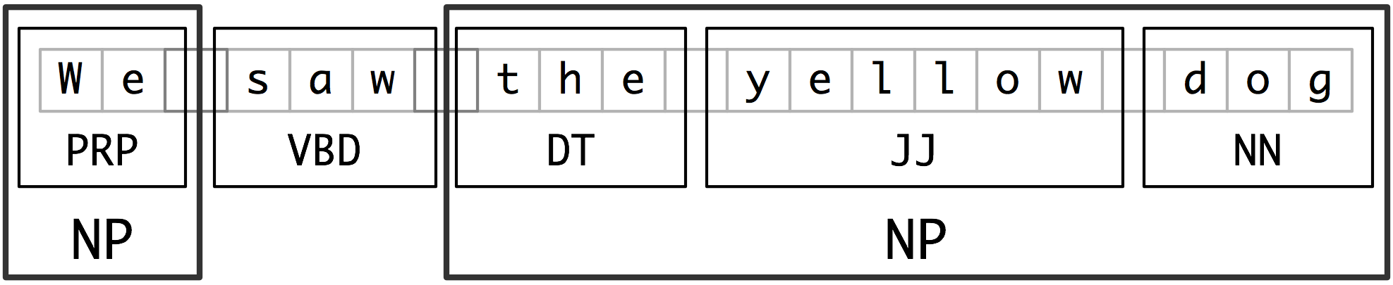
        • Noun-phrase (NP) chunking
        • tag patterns: describe sequences of tagged words
        • Chunking with Regular Expressions
        • Exploring Text Corpora
      • Chinking: define a chink to be a sequence of tokens that is not included in a chunk
      • Representing chunks: tags & trees
      • Training Classifier-Based Chunkers
  • Accurate methods for the statistics of surprise and coincidence
• An introduction to lexical association measures:
  • We use the term lexical association to refer to the association between words.
  • 3 types of association:
    • collocational association: restricting combination of words into phrases
    • semantic association: reflecting the semantic relationship between words
    • d cross-language association: corresponding to potential translations of words between different languages
• Topics:
  • Knowledge/ data->zipf
  • Hypothesis testing
  • Collations
  • NER
• Knowledge/ data
  • Rationalist:
  • Empiricist: driven by observation
  • Zipf’s law: the frequency of any word is inversely proportional to its rank in the frequency table.
    •                                      Empiricist                          Rationalist
    • core                              frequent
    • periphery                     infrequent                     exception relation
  • Example 1
    • Alice like it. a book.
    • Question: what does Alice like?
    • Instead of using a string of word, use a tree structure to represent a sentence.
    •              CP
    •    spec           IP
    • what         Alice like
  • Example 2 (Rationalist)
    • Which book did mary say that Bill thinks Alice like?
    • He dropped a book about info theory.
    • What did he drop a book about? (questionable) What did he write a book about? (Good)
    • He dropped [a book about info theory].
    • S                                   NP
  • Example 3
    • What does Mary read?
    •        SBarQ
    • WhNP                             SQ
    • WP           VR           NP             VBR                   NP
    •  what         odes     mary              read                  T*-1
  • Balance between rationalist and empiricist
  • Accuracy vs. coverage
  • Data-driven algorithms less concerned with over generation
  • Semi-supervised learning
  • How to relate the algorithm to the wat we learned.
  • 80-20 rule
  • Remove the low-frequency word and focus on the frequent words for the structure.
• Hypothesis testing (Chi^2 test)
  • P(H|E) H: hypothesis, E: evidence
  • P(q = 0.7 | 76 success, 24 failures)
  • pmf:
  • R = P(H1|E) / P(H2|E)
  • Recipe for statistical hypothesis
    • Step 1: H0: null hypothesis (what we think is not true)
      • Example: coin flip: coin has only one side.
    • Step 2: Test statistic: number we compute based on evidence collection
    • Step 3: Identify test statistics distribution: if H0 were true.
    • Step 4: Pick a threshold to convince that the H0 is not true.
    • Step 5: Do an experiment and calculate the test statistic.
    • Step 6: If it sufficiently improbable assuming H0 is true, should reject H0.
      • H0: q = 0.05, H1: q != 0.05
  • Example:
    • H0: P(H) = 0.05
    • R~Binomial(n, p)
    • Likelihood func: b(r,n,p) = C(n r) p^r (1-p)^(n-r)
    • Test statistics: # heads
    • Threshold:
      • alpha = 10e-10 Type II: “miss”, “false negative”
      • alpha = 0.2 Type I: “false positive”
      • Typically, people choose alpha = 0.05
    • The value on the edge (alpha = 2.5%) is critical value.
    • Tips:
      • alpha is selected in advance. (p-hacking)
      • Cannot be used to prove something is true, only can show that something is not true.
      • Chi^2? X^2
  • Difference between Chi^2 test and T-test
  • How do I know how many times of experiment is convincing?
  • Collocation:  collocation is a sequence of words or terms that co-occur more often than would be expected by chance.
    • Kict the bucket = to die

• Question2:
  • Word order:
    • Explanation: Word order refers to the structure of a sentense:
      • Alexa, when is your birthday?
      • (Alexa answers)
      • Alexa, when your birthday is?
      • (Alexa answers)
      • This will test whether alexa handles some wrong word order.
  • Inflectional morphology:
    • Explanation:
• Question 3:
• Question 4:
  • Reference: http://statweb.stanford.edu/~serban/116/bayes.pdf
• Question 5:
• Question 6:
  • New definitions:
    • log-entropy weighting
    • cosine similarity

• Dependency Parsing
  • Dependency: focuses on relations between words
    • Typed: Label indicating relationship between words
    • Untyped: Only which words depend
  • Phrase structure: focuses on identifying phrases and their recursive structure
  • Dependency parsing methods:
    • Shift reduce:
      • Predict from left to right
      • Fast, but slightly less accurate
      • MaltParser
    • Spanning tree:
      • Calculate full tree at once
      • Slightly more accurate, slower
      • MSTParser, Eda
    • Cascaded chunking
      • Chunk words into phrases, find heads, delete non-heads, repeat
      • CaboCha
  • Example
    • Maximum Spanning Tree
      • Each dependency is an edge in a directed graph
      • Assign each edge a score
      • Keep the tree with the highest score
    • Cascaded Chunking

      For Japanese
    • Shift-Reduce
      • Two data Structures:
        • Queue: of unprocessed words
        • Stack: of partially processed words
      • Process: at each point, choose”
        • Shift: move one word from queue to stack
        • Reduce left: top word on stack is head of second word
        • Reduce right: second word on stack is head of top word
      • Classification for shift-reduce
        • We have a weight vector for “shift” “reduce left”,“reduce right”: Ws, Wl, Wr
        • Calculate feature functions from the queue and stack: φ(queue, stack)
        • Multiply the feature functions to get scores: Ss = Ws * φ(queue, stack)
        • take the highest score and choose the function
      • Features for Shift Reduce:
        • Features should generally cover at least the last stack entries and first queue entry
      • Algorithm:
        • Input:
          • weights:Ws, Wl, Wr
          • queue: [(1 word1, Pos1), (2, word2, Pos2), …]
          • stack: [(0, ROOT, ROOT)]
        • Output:
          • heads = [-1, head1, head2, …]
        • Pseudo Code
        • Training
          • Can be trained using perceptron algorithm
          • Do parsing, if correct answer, corr different from classifier answer ans, update weights
          • Shift-reduce training algorithm
  • CKY (Cocke-Kasami-Younger) Parsing Algorithm & Earley Parsing Algorithms
    • Definitions:
      • CFG (Context-free Grammar): G = (N, Σ, P, S)
        • N is a finite set of non-terminal symbols
        • Σ is a finite set of terminal symbols (tokens)
        • P is a finite set of productions (rules)
          • Production : (α, β)∈P will be written α → β where α is in N and β is in (N∪Σ)*
        • S is the start symbol in N
      • CNF (Chomsky Normal Form):
        A context-free grammar where the right side of each production rule is restricted to be either two non terminals or one
        terminal. Production can be one of following formats: A->a || A->BC.

        Any CFG can be converted to a weakly equivalent grammar in CNF
    • Parsing Algorithms:
      • Should know:
        • CFGs are basis for describing (syntactic) structure of NL sentences
        • Parsing Algorithms are core of NL analysis systems
        • Recognition vs. Parsing:
          • Recognition-deciding the membership in the language
          • Parsing–Recognition+ producing a parse tree for it
        • Parsing is more “difficult” than recognition (time complexity)
        • Ambiguity-an input may have exponentially many parses.
      • Top-down VS Bottom-up
        • Top-down (goal driven): from start symbol down
        • Bottom-up (data driven): from the symbols up
      • Naive vs. dynamic programming
        • Naive: enumerate everything
        • Back tracking: try something, discard partial solutions
        • DP: save partial solutions in a table
      • CKY: Bottom-up DP
      • Earley Parsing: top-down DP
  • Chart Parsing:
  • Lambda Calculus
  • Perceptron Learning
  • Restricted Boltzmann Machines
  • Statistical Hypothesis Testing
  • Latent Semantic Analysis
  • Latent Dirichlet Allocation
  • Gibbs Sampling
  • Inter-rater Reliability
  • IBM Models for MT
  • Phrase-based Statistical MT
  • Hierarchical Phrase-based Statistical MT
  • Lambda Reductions
  • Probabilistic Soft Logic
  • Open Information Extraction
  • Semantic Role Labeling
  • Combinatory Categorial Grammar (CCG)
  • Tree Adjoining Grammar
  • Abstract Meaning Representation (AMR)
  • Wikification

Challenges:

1. Mathematical representation of model
2. learning models parameters from data

Overview:

• generative face model
  • space of faces: goals
    • each face represented as high dimensional vector
    • each vector in high dimensional space represents a face
  • Each face consists of
    • shape vector Si
    • Texture vector Ti
  • Shape and texture vectors:
    • Assumption: known point to point corrsp between faces
    • construction: for eaxample 2D parameterization using few manually selected feature points
    • shape, texture vecs: sampled at m common locations in parameterization
      • Typically m = few thousand
      • shape texture vecs 3m dimensional (x, y, z & r, g, b)
      • *feature points may not be sampled.
  • linear face model
    • linear combinations of faces in database
      • s = sum(ai * Si)
      • t = sum(bi * Ti)
      • Basis vectors Si, Ti
      • Avg face Savg = 1/n sum(Si)
      • Avg face Tavg = 1/n sum(Ti)
  • Probabilistic modeling
    • PDF over space of faces gives probability to encounter certain face in a population
    • Sample the PDF generates random new faces.
    • Ovservation
      • Shape & tex vecs are not suitable for probabilistic modeling
      • Too much redundancy
      • many vecs do not resemble real faces
      • real faces occupy
    • AssumptionL faces occupy linear subspace of high dimensional space.
      • Faces lie on hyperplane
      • Illustration in 3D
        • faces lie on 2D plane in 3D
      • How to determine hyperplane?
        • PCA:
          • find orthogonal sets of vecs that best represent input data points
          • first basis vec: largest variance along its direction
          • Following basis vecs: orthogonal, ordered according to variance along their directions
        • Dimensionality reduction:
          • discard basis vectors with low variance
          • represent each data point using remaining k basis vecs (k-dim hyperplane)
          • can show: hyperplanes obtained via PCA minimize L2 distance to plane
        • First basis vec maximized variance along its direction
          • w{1} = argmanx{sum((t1)i^2)} – argmax sum(xi * w)^2 = argmax{||Xw||^2} = argmax{w’X’Xw}
          • data points as row vecs xi , zero mean
          • matrix X consists of row vecs xi
        • w{1} is the eigenvec corespp to the max eigenvalue of X’X
      • Properties;
        • Matrix X’X is proportional to so-called sample covariance matrix of dataset X
        • if dataset has multi-variance normal distribution, maximum likelihood estimation of distribution is
          • f(x) = (2* pi) ….
      • Node
        • X is very large X is n x m matrix
          • n is # data vec
          • m is length of data vec
        • m>> n in general
        • X is m x m matrix, very large
      • SVD of X
        • X = U sigma V’
        • X’X  = V sigma’ UU’ sigma V’ = V sigma^2 V’
        • right singular vecs V of X are eigenvec of X’X
        • singular values sigma(k) of X are square roots of eigenvalues lambda(k) of X’X
        • change of bassis into orthogonal PCA basis by projection onto eigenvectors
      • T = XV = Usigma V’V = uSigma
      • left singular vectors U multiplied by singular velues in sigma
    • Dimensionality reduction
      • only consider l eigenvectors/ singular vectors correp to l largest singular values
      • Tl = XVl = U l * sigma l
      • Matrix Tl in R (mxl)  contains coord of m samples in reduced number l of dim
      • computation of only l components directly via truncated SVD
      • multivariate normal distribution in reduced space has covariance matrix
      • Diagonal matrix, l largest eigenvalues of X’X
      • PCA diagonalizes covariance matrix decorrelates data
  • attribute based modeling
    • mnually define attributes, label each face i with a weight mui for each attribute mu
    • attribute vecs
    • add/ subtract multiple of attribute vecs
  • model fitting, tracking
    • Assume a parametric shape model
      • Given parameters,can generate shape
    • model fitting, tracking problem
      • given some observation, find shape
      • parameters that most likely to produce the observation
    • bayes theorem
  • Matching to images
    • Model parameters to generate an image
      • Shape vec: alpha
      • tex vec: beta
      • rendering parameters (projection, lighting) rou
    • Given image, what are the most likely rendering parameters that generate that image
      • MAP
      • BAyes
      • compute max p
• Discussion
  • adv:
  • Disadv:
    • linear mdoel may not be accurate
    • linear model not suitable for large geometric deformations (rotations)

• Reference
  • http://www.pmp-book.org/download/slides/Deformation.pdf
  • https://zhuanlan.zhihu.com/p/25804146
• Deformation energy
  • Geometric energy to strtch and band thin shell from one shape t another as difference between first and second fundamental form
    • First: stretching
    • second: bending
  • Approach:
    • Given constraints (handle position / orientation, find surface that min deformation energy)
  • Linear Approximation
    • Energy based on fundamental forms in non-linear function of displacements
      • Hard to minimize
    • linear approximation using partial derivatives of displacement function.
      • Assume parameterization of displacement field d(u,v)
      • Bending:
        • linear energy:
          • laplace = 0 minimize surface area
        • Variational calculus, Euler0-Lagrange equations:
          • laplace of laplace: make it smooth (the derivative of surface change continuously and is minimized)
        • So, apply bi-laplacian on mesh
  • Skeletal animation